The median values for the beginning heights, heights of maximum brightness and ending heights have been obtained for sporadic meteors and for meteors of the IAU established meteor shower list, based on the CAMS dataset 2010–2013. Two layers with larger numbers of events with in between a layer with significant less events were found. A seasonal variation in the geocentric velocity and ablation height for sporadic meteors has been found with maximum values for the median height around solar longitude 225° and minima around 45°. For individual shower meteors there is a significant number of showers that produce meteor trajectories below the 90 km level. To avoid any bias that may affect the number of orbits collected for slower meteors, the 80 km level is recommended as reference level to optimize the pointing of the cameras in the BeNeLux CAMS network.
1 Introduction
The CAMS network uses a standard configuration at each station for both the hardware as well as for the software. The equipment consists of a Watec H2 Ultimate video camera with a Pentax 1.2/12mm lens. The field of view is rather small with about 30° × 22°. This allows capturing fainter meteors and offers a better accuracy than large FoV optics. Initially the concept of the CAMS project was to have all-sky coverage by the combination of 20 cameras at a single station that function as a mosaic of slightly overlapping FoVs, comparable to a facette eye of an insect (Jenniskens et al., 2011).
The first stand-alone single-CAMS were pointed at the sky as extra coverage for the all-sky set-ups in California. Where single-CAMS were applied without any coverage from some main all-sky set-up, the number of simultaneously captured meteors depended on the intersection of the camera fields at a height where most meteors can be expected. To have an optimal number of coincidences, the aiming points for the cameras must be carefully chosen in function of favorable geometrics and an optimal overlap. For this purpose the camera fields are projected on a plane at a chosen height, parallel to the Earth surface. The main question is; at which height can we expect to capture most meteors and how can we be sure to cover the entire population of sporadic and shower meteors without introducing any bias?
2 Camera fields and meteor heights
The volume of the atmosphere that a camera covers increases with the height in the atmosphere. At a level of 100 km we cover significant more square kilometers than at lower heights and therefore some people prefer to organize the camera fields at this range in order to have the largest number of square kilometers covered. However the majority of all meteors is to be detected below 100 km in the atmosphere and some of these meteors risk to be missed at lower elevation in between camera fields. In the past we have been working with 90 km as reference level to overlap camera fields for CAMS, but is this the best option?
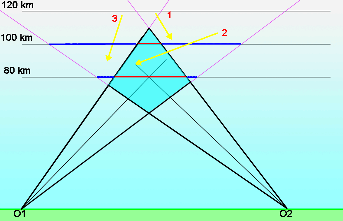
The level at which the camera fields are optimized should be carefully chosen. The higher in the atmosphere, the larger the volume covered and thus less cameras are necessary to cover such part of the atmosphere (see Figure 1). But if the height at which meteors appear is variable throughout the year or proves to be different from one shower to another, then some bias could be created in the sense that part of the meteors that produce their luminous trails at lower heights have less chance to be captured. With other words, part of the meteors will get lost in the uncovered ‘gaps’ between the camera fields. As a result less orbits will be collected for meteors that appear deeper in the atmosphere, being discriminated by the selection of the optimal level to aim the cameras. In the end the dataset of orbits will not be representative for the total meteor population.
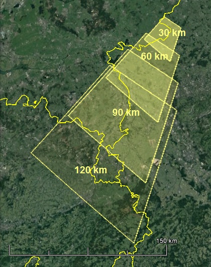
Figure 1 – A FoV of 30° × 22° aimed at an azimuth of 211° and a height of 41° with a tilt of 5.6° intersected with a plane at 30 km, 60 km, 90 km and 120 km.
For a wide expanded and dense camera network such as the BeNeLux network any good combination at a level of 80 km will be even better covered at higher levels by cameras from other stations that reach deeper in the atmosphere at higher levels (see Figure 2). This is not true when only few cameras are available at too few stations as in such case the camera fields will overlap at the reference level and diverge at higher levels (see Figure 3).
For the BeNeLux network we need to know how the heights of meteors are distributed in the atmosphere to determine the best level at which the camera intersections must be optimized.
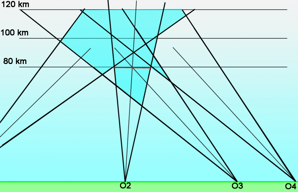
Figure 2 – When a camera network has enough cameras at many participating stations, the number of simultaneous meteors can be increased by optimizing the volume covered from different stations. The level to optimize overlap is important to know. If well covered at lower height, e.g. 80 km, more overlap will be generated by cameras that are further away.

Figure 3 – Observers O1 and O2 aiming their cameras at a common point at 80 km height in the atmosphere will capture only simultaneously meteors in their common volume in the atmosphere. Meteors 1 and 2 will appear nice in the picture of O1, and meteor 3 and part of meteor 2 in the picture of O2, but only part of meteor 2 will be double station.
3 Meteor heights in the atmosphere
A while ago Pete Gural asked the author to remake the CAMS shower reference list which was based on the IMO Shower Calendar. The purpose is to create a new reference list as source for some future new tools in the CAMS software. It was decided that the new reference list should be based on the IAU Established Meteor Shower List. Some of the shower characteristics that are needed are the heights of beginning, ending and maximum brightness for each shower. The previously used values were taken from IMO where these values had been copied through different editions from research work from the 1960s (Jacchia et al., 1967). With the public available CAMS dataset of 111233 orbits obtained in 2010–2013 (Jenniskens et al., 2016), we have a reliable source to derive statistics on the heights of the calculated trajectories.
We counted the number beginning heights in layers of 5 km thickness each, e.g. higher than 60 km and less than or equal to 65 km, counting this way for all 5 km thick layers until the layer >125 km and <=130 km. Only 0.2% of all meteors started below 75 km elevation and only 0.2% above 125 km. About all beginning points appear in the 50 km thick atmospheric zone between 75 and 125 km height. Doing this for the heights of greatest luminosity and for the end points, the overall majority proves to be situated above 70 km and below 115 km height in the atmosphere. Results are listed in Table 1 and Figure 4.
There is a strange feature in Table 1 as there are significant more meteors starting between 105–115 km height and between 90–100 km than in between at 100 and 105 km. This effect can also be noticed in the counts for the height of the brightest luminosity (less between 95 and 100 km, and the ending points (less between 90 and 95 km. There is no straightforward explanation for this effect. Major meteor streams cannot really account for this as only 27.6% of the dataset concerned shower meteors, none of which had a particular big weight in the statistics. A possible explanation could be an artifact as a bias in the CAMS configuration that favors detection of double station meteors at certain elevations unless some physical difference in the atmospheric layers occurs.
Table 1 – Number of trajectories for all layers of 5 km thick from 60 km until 130 km height.
| km | Start | Brightest | End | |||
| <=60 | 8 | 0.0% | 34 | 0.0% | 143 | 0.1% |
| 60-65 | 2 | 0.0% | 56 | 0.1% | 222 | 0.2% |
| 65-70 | 17 | 0.0% | 264 | 0.2% | 907 | 0.8% |
| 70-75 | 235 | 0.2% | 1275 | 1.2% | 2907 | 2.6% |
| 75-80 | 1772 | 1.6% | 3891 | 3.5% | 7873 | 7.1% |
| 80-85 | 4092 | 3.7% | 9140 | 8.3% | 17015 | 15.4% |
| 85-90 | 7043 | 6.4% | 18447 | 16.7% | 22226 | 20.1% |
| 90-95 | 14283 | 12.9% | 20049 | 18.1% | 17739 | 16.1% |
| 95-100 | 21564 | 19.5% | 15688 | 14.2% | 21451 | 19.4% |
| 100-105 | 13656 | 12.4% | 22838 | 20.7% | 16558 | 15.0% |
| 105-110 | 19156 | 17.3% | 16095 | 14.6% | 3234 | 2.9% |
| 110-115 | 21690 | 19.6% | 2628 | 2.4% | 230 | 0.2% |
| 115-120 | 5893 | 5.3% | 109 | 0.1% | 16 | 0.0% |
| 120-125 | 889 | 0.8% | 6 | 0.0% | 0 | 0.0% |
| 125-130 | 169 | 0.2% | 0 | 0.0% | 0 | 0.0% |
| >130 | 52 | 0.0% | 1 | 0.0% | 0 | 0.0% |
| 110521 | 100.0% | 110521 | 100.0% | 110521 | 100.0% | |
In a private communication Dr. Peter Jenniskens explains the dip as a distinct difference of the Apex and Anti Helion sources. The Apex contributes fast meteors 50-75 km/s, the Anti Helion very slow meteors 12–40 km/s. The dip is situated at 40-50 km/s, which is also visible in the height distribution of meteor trajectories.
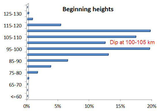
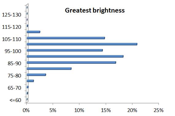
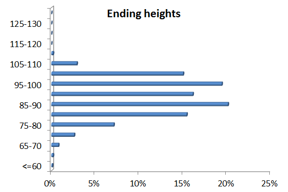
Figure 4 – Graphical presentation of the values of Table 2. The distribution of beginning heights (top), heights of greatest brightness (middle) and the ending heights (bottom) display a remarkable dip in the height distribution. Not any major shower has enough weight in the sample to explain this effect.
4 Seasonal variations for sporadics
79990 orbits concerned sporadics. In an attempt to verify if any seasonal variations could be detected, the dataset was split into 12 intervals, each covering 30° in solar longitude. For each interval the median has been calculated for the beginning height, the height of maximum brightness and the ending height. The results are listed in Table 2. Since all individual meteor orbits in CAMS were validated according to strict quality control criteria, these statistics should be reliable.
From Table 2 it is obvious that the characteristics of the sporadic background show some variation. Around the time of solar longitude 225° the median geocentric velocity of the sporadic background is significant faster with 57.4 km/s than at the opposite position of the Earth on its orbit at solar longitude 45° where the median geocentric velocity is 32.7 km/s (Figure 5). The ablation height of a meteor depends on the energy with which it enters into the atmosphere, the higher the velocity the higher the potential energy for a given mass. Fast meteors produce their luminous trajectory much higher in the atmosphere than slow meteors. The reason why the sporadics background appears to be slower around a solar longitude of 45° and faster around 225° is not clear. Perhaps the sporadic background around solar longitude 225° was composed from ancient trails of dispersed dust, left over from unknown long periodic comets such as P/Halley? According to Dr. Peter Jenniskens the elevation of the Apex may be an explanation as main source of fast meteors. Question is if the Southern hemisphere has the opposite effect? Note that the visibility of the Apex is the same at the Spring and at the Autumn equinox, while the median velocity of sporadic meteors is very different.
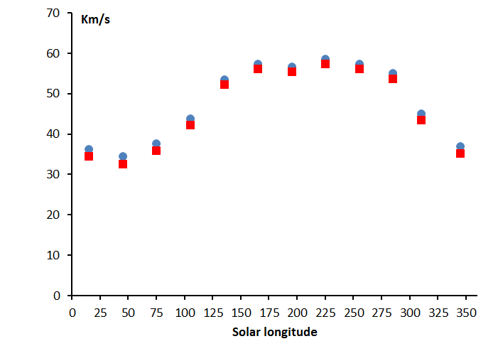
Figure 5 – The variation of the median velocity in function of the solar longitude. The blue dot is the median entry velocity and the red square the median geocentric velocity.
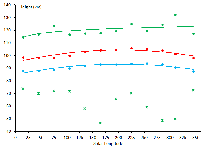
Figure 6 – The median values for sporadic meteors for the starting height (green), the height of maximum luminosity (red), the ending height (blue) and the lowest starting height recorded as outlier in each time span (green x).
Whatever the cause is for this seasonal variation in the velocity and ablation height, we should optimize our camera network in such a way that we create no bias by missing too many slower meteors deeper in the atmosphere. From the median values and standard deviation we can conclude that we should cover the atmospheric layer from about 110±10 to 90±10 km (see Table 2 and Figure 6). Interested in all meteors, also the outliers, I included the most extreme values found for each interval. These individual cases show that some meteors ablate far above or below the preferable elevation in the atmosphere. To choose an optimal level in the atmosphere to capture as many of these meteors as possible is a tradeoff, between the number of available cameras to cover a layer in the atmosphere and the number of outliers that can be ignored.
The CAMS dataset allowed to check for seasonal variations within a calendar year but does not yet cover enough years to check for long term variations in ablation heights. Such variations have been reported before in radar data and were supposed to be linked with the 11 year periodicity of the solar activity, but this is not proven yet and the topic needs further investigation (Porubčan et al., 2012).
Table 2 – Heights in the atmosphere (km) for sporadic meteors, with Hb the starting height, Hm the height of maximum brightness, He the ending height, Vg the geocentric velocity and N the number of trajectories in the sample.
| λʘ | Hb | Hb max |
Hb min |
Hm | Hm max |
Hm min |
He | He max |
He min |
Vg | N |
| 0 – <30 | 98.6±10.3 | 125.8 | 73.8 | 92.2±9.2 | 114.4 | 57.1 | 87.9±9.1 | 114.4 | 49.7 | 34.5 | 2366 |
| 30 – <60 | 98.3±10.1 | 129.5 | 69.9 | 92.1±9.2 | 116.9 | 55.9 | 88.0±8.8 | 111.6 | 47.8 | 32.7 | 4355 |
| 60 – <90 | 98.0±9.8 | 129.8 | 72.1 | 92.2±9.1 | 123.7 | 51.9 | 88.6±8.6 | 119.5 | 47.7 | 35.9 | 4821 |
| 90 – <120 | 100.0±10.0 | 131.5 | 71.6 | 94.2±9.2 | 116.6 | 56.8 | 89.9±8.7 | 114.2 | 50.8 | 42.3 | 7355 |
| 120 – <150 | 103.0±9.7 | 132.3 | 58.0 | 96.7±9.0 | 117.5 | 50.6 | 91.8±8.6 | 115.0 | 46.8 | 52.4 | 9454 |
| 150 – <180 | 104.2±9.7 | 139.7 | 46.6 | 97.7±8.9 | 117.7 | 43.4 | 93.0±8.8 | 114.2 | 37.5 | 56.2 | 7277 |
| 180 –<210 | 104.3±10.2 | 136.1 | 65.7 | 97.9±9.4 | 119.4 | 50.0 | 93.0±9.0 | 117.5 | 46.0 | 55.5 | 7691 |
| 210 – <240 | 105.8±10.4 | 154.5 | 70.1 | 98.7±9.8 | 124.9 | 63.6 | 93.7±9.5 | 116.4 | 49.9 | 57.4 | 7762 |
| 240 – <270 | 105.3±10.4 | 136.2 | 58.9 | 98.7±9.7 | 119.5 | 53.4 | 93.8±9.5 | 117.7 | 46.6 | 56.2 | 8890 |
| 270 – <300 | 104.0±10.6 | 143.4 | 48.7 | 97.9±9.7 | 124.4 | 46.4 | 93.2±9.6 | 117.9 | 40.8 | 53.8 | 10338 |
| 300 – <330 | 101.1±10.5 | 137.3 | 49.9 | 94.9±9.8 | 132.2 | 53.1 | 90.6±9.7 | 114.5 | 44.6 | 43.6 | 6018 |
| 330 – <360 | 98.1±10.4 | 127.4 | 72.5 | 91.8±9.5 | 117.3 | 64.9 | 87.5±9.2 | 114.7 | 56.2 | 35.3 | 3663 |
| All spor. | 102.2±10.3 | 154.5 | 46.6 | 96.2±9.5 | 132.2 | 43.4 | 91.5±9.2 | 119.5 | 37.5 | 47.5 | 79990 |
| All streams | 101.6±8.3 | 142.7 | 74.5 | 94.7±8.1 | 118.4 | 54.2 | 90.2±7.9 | 116.4 | 40.7 | 41.6 | 29513 |
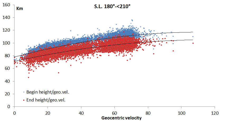
Figure 7 – Plot of individual meteor heigths, beginning and ending heights in function of the geocentric velocity for all meteors registered within the period 180°>= λʘ< 210°. This graph shows that the ablation heights increase in function of the geocentric velocity.
5 Established meteor showers
Table 3 – Heights in the atmosphere (km) for meteors of the IAU established meteor shower list, with Hb the starting height, Hm the height of maximum luminosity, He the ending height, Vg the geocentric velocity and N the number of trajectories in the sample.
| IAU code | Hb | Hb max |
Hb min |
Hm | Hm max |
Hm min |
He | He max |
He min |
Vg | N |
| KSE – 27 | 104.7±6.2 | 113.8 | 87.9 | 96.1±5.6 | 102.6 | 82.1 | 89.0±5.7 | 99.8 | 74.4 | 46.7 | C21 |
| AVB – 21 | 95.1±1.6 | 96.2 | 90.7 | 86.4±2.8 | 92.2 | 81.3 | 83.9±4.2 | 89.1 | 72.7 | 18.8 | C12 |
| LYR – 6 | 107.3±4.7 | 136.5 | 91.4 | 99.7±4.8 | 109.0 | 76.9 | 93.2±5.4 | 104.4 | 71.7 | 46.7 | C257 |
| ARC – 348 | 102.8±3.8 | 109.9 | 89.3 | 97.0±3.2 | 102.7 | 86.3 | 92.6±3.9 | 99.5 | 80.8 | 40.9 | C42 |
| HVI – 343 | 89.7±5.7 | 99.7 | 84.1 | 85.7±5.6 | 96.5 | 78.6 | 80.8±5.9 | 92.3 | 75.1 | 17.2 | C11 |
| ETA – 31 | 113.6±3.6 | 129.7 | 98.3 | 106.6±3.3 | 116.6 | 92.2 | 100.6±4.1 | 115.9 | 87.0 | 65.7 | C936 |
| NOC – 152 | 102.8±2.2 | 103.7 | 98.9 | 98.0±2.4 | 100.5 | 95.5 | 93.3±1.9 | 95.7 | 91.0 | 36.2 | C4 |
| ELY – 145 | 105.5±3.3 | 113.8 | 95.5 | 96.8±4.7 | 107.5 | 84.6 | 92.1±4.7 | 101.3 | 83.5 | 43.7 | C39 |
| EAU – 151 | 92.5±2.1 | 97.4 | 90.9 | 89.7±2.5 | 96.2 | 88.0 | 85.8±3.3 | 92.4 | 82.8 | 31.5 | C11 |
| JMC – 362 | 104.5±5.2 | 112.0 | 91.8 | 96.9±4.3 | 107.4 | 90.0 | 93.2±4.4 | 100.3 | 84.8 | 41.7 | C32 |
| ARI – 171 | 100.7±2.1 | 104.4 | 96.2 | 97.6±2.7 | 102.3 | 90.1 | 93.8±3.6 | 99.8 | 87.1 | 41.1 | C31 |
| JRC – 510 | 110.1±3.9 | 118.4 | 104.7 | 101.1±4.7 | 107.8 | 91.5 | 93.1±4.0 | 98.8 | 86.2 | 50.9 | C14 |
| BEQ – 327 | 93.4±3.0 | 103.2 | 88.8 | 89.4±2.2 | 96.8 | 86.4 | 85.6±1.9 | 90.7 | 81.6 | 33.2 | C38 |
| SSG – 69 | 97.3±2.9 | 103.3 | 87.7 | 92.4±2.9 | 101.3 | 84.9 | 89.9±3.1 | 99.6 | 81.1 | 25.1 | C70 |
| COR – 63 | 79.1±4.5 | 87.8 | 75.4 | 74.0±5.2 | 84.3 | 67.8 | 71.6±6.5 | 82.8 | 60.1 | 8.7 | C12 |
| EPR – 324 | 106.3±1.4 | 107.7 | 104.3 | 99.2±2.6 | 104.3 | 98.9 | 95.2±3.4 | 101.4 | 94.2 | 43.8 | C4 |
| JIP – 431 | 113.0±5.6 | 128.2 | 106.8 | 102.7±4.6 | 105.6 | 90.4 | 96.3±4.8 | 103.2 | 84.8 | 58.5 | C11 |
| NZC – 164 | 95.9±3.0 | 107.3 | 87.3 | 91.3±2.5 | 99.5 | 78.5 | 86.8±2.9 | 94.6 | 65.6 | 38.3 | C404 |
| PPS – 372 | 112.5±3.2 | 123.5 | 97.0 | 105.9±3.7 | 116.0 | 88.3 | 100.2±4.2 | 114.9 | 87.0 | 66.5 | C379 |
| SZC – 165 | 96.9±3.0 | 106.3 | 91.3 | 93.1±2.6 | 102.1 | 86.4 | 88.4±2.8 | 98.4 | 82.7 | 39.2 | C89 |
| CAN – 411 | 108.8±3.3 | 117.2 | 95.7 | 101.3±3.8 | 110.1 | 89.8 | 96.3±4.3 | 109.3 | 82.3 | 57.5 | C169 |
| EPG – 326 | 92.4±2.3 | 98.8 | 89.3 | 89.1±2.6 | 96.3 | 83.6 | 85.7±2.8 | 90.3 | 79.9 | 28.4 | C33 |
| ALA – 328 | 97.8±7.2 | 102.9 | 92.7 | 93.8±7.4 | 99.0 | 88.6 | 88.4±5.4 | 92.2 | 84.6 | 37.4 | C2 |
| JXA – 533 | 114.4±3.7 | 121.7 | 107.7 | 103.3±3.8 | 112.5 | 97.5 | 96.6±4.6 | 111.1 | 92.1 | 68.9 | C20 |
| JPE – 175 | 111.4±4.0 | 124.3 | 95.9 | 102.5±3.8 | 110.8 | 89.6 | 97.6±4.0 | 106.6 | 84.1 | 64.0 | C104 |
| FAN – 549 | 111.2±3.9 | 123.7 | 99.7 | 104.9±4.9 | 114.1 | 85.5 | 98.2±4.7 | 107.5 | 81.8 | 60.2 | C76 |
| PCA – 187 | 98.5±5.3 | 111.6 | 91.2 | 92.8±3.9 | 101.3 | 85.8 | 88.3±3.4 | 96.7 | 82.8 | 42.0 | C36 |
| GDR – 184 | 98.3±2.6 | 103.9 | 93.4 | 90.3±3.1 | 96.7 | 83.8 | 86.5±3.1 | 91.0 | 78.1 | 27.5 | C40 |
| CAP – 1 | 96.2±2.4 | 104.6 | 84.3 | 89.8±3.1 | 99.0 | 73.5 | 86.5±3.4 | 93.4 | 69.8 | 23.0 | C646 |
| SDA – 5 | 97.1±2.6 | 106.9 | 88.9 | 93.3±2.4 | 103.7 | 79.8 | 87.7±2.8 | 103.3 | 72.2 | 41.3 | C1382 |
| PAU – 183 | 97.0±3.6 | 104.9 | 92.0 | 93.9±2.6 | 99.6 | 88.5 | 89.4±2.9 | 94.4 | 84.8 | 43.9 | C23 |
| ERI – 191 | 112.1±3.7 | 129.8 | 97.8 | 105.6±3.7 | 116.0 | 92.7 | 101.3±4.4 | 111.2 | 81.3 | 64.5 | C214 |
| PER – 7 | 110.9±4.0 | 142.7 | 89.4 | 103.0±4.6 | 116.7 | 79.6 | 98.0±4.8 | 115.8 | 65.8 | 59.1 | C4366 |
| NDA – 26 | 96.1±3.0 | 104.0 | 89.5 | 91.8±2.6 | 101.2 | 82.7 | 87.0±2.9 | 96.8 | 79.3 | 38.4 | C251 |
| KCG – 12 | 93.7±2.4 | 98.1 | 88.5 | 86.5±4.5 | 95.1 | 71.1 | 84.2±4.6 | 88.0 | 68.2 | 20.9 | C25 |
| AUD – 197 | 95.1±2.9 | 97.4 | 85.2 | 86.3±2.3 | 89.7 | 81.5 | 83.9±3.4 | 88.0 | 74.2 | 21.1 | C17 |
| NIA – 33 | 96.2±4.3 | 106.3 | 83.7 | 89.6±3.9 | 99.0 | 79.5 | 85.6±3.7 | 95.8 | 78.3 | 31.3 | C94 |
| AUR – 206 | 111.5±3.7 | 119.4 | 103.4 | 105.4±4.8 | 114.1 | 92.5 | 101.9±5.5 | 113.7 | 89.6 | 65.6 | C19 |
| SPE – 208 | 111.9±5.1 | 131.3 | 102.7 | 102.9±5.1 | 111.0 | 87.4 | 97.8±5.0 | 106.0 | 83.5 | 64.8 | C291 |
| NUE – 337 | 112.7±4.1 | 130.5 | 96.2 | 106.3±4.1 | 116.1 | 90.4 | 101.3±4.5 | 114.2 | 83.4 | 67.1 | C85 |
| DSX – 221 | 98.4±2.5 | 105.1 | 96.3 | 93.0±3.5 | 99.9 | 88.9 | 90.4±4.6 | 98.0 | 81.5 | 32.9 | C14 |
| DRA – 9 | 97.8±2.2 | 102.6 | 94.7 | 93.8±3.1 | 99.0 | 87.7 | 90.1±3.4 | 94.6 | 81.0 | 20.7 | C30 |
| EGE – 23 | 113.4±3.1 | 118.8 | 103.3 | 104.0±4.2 | 113.8 | 96.5 | 97.8±3.6 | 109.7 | 92.3 | 69.6 | C31 |
| OCU – 333 | 115.4±5.3 | 119.1 | 102.0 | 106.3±3.3 | 110.9 | 100.4 | 97.0±3.6 | 101.2 | 91.7 | 55.6 | C9 |
| ORI – 8 | 113.1±3.6 | 133.9 | 96.1 | 105.6±4.0 | 118.4 | 79.5 | 99.4±4.1 | 116.4 | 77.1 | 66.3 | C3024 |
| LMI – 22 | 115.4±4.6 | 124.1 | 102.3 | 107.9±4.4 | 115.6 | 88.2 | 98.3±4.2 | 110.4 | 87.5 | 61.9 | C64 |
| LUM – 524 | 114.2±3.9 | 117.0 | 108.5 | 106.5±7.9 | 108.0 | 91.3 | 99.0±5.1 | 103.0 | 90.8 | 60.9 | C4 |
| STA – 2 | 97.4±3.8 | 109.5 | 82.2 | 88.7±4.3 | 101.0 | 63.4 | 84.4±4.9 | 98.8 | 59.0 | 26.6 | C916 |
| NTA – 17 | 97.5±3.8 | 110.4 | 83.6 | 88.3±4.6 | 105.0 | 65.3 | 83.8±5.0 | 98.5 | 60.7 | 28.0 | C509 |
| CTA – 388 | 96.4±4.0 | 104.8 | 88.6 | 91.1±4.2 | 100.1 | 79.3 | 86.4±4.3 | 97.4 | 72.1 | 41.1 | C52 |
| SLD – 526 | 109.6±4.6 | 113.8 | 94.6 | 104.5±4.6 | 109.4 | 94.0 | 98.0±4.3 | 103.2 | 88.4 | 49.1 | C13 |
| OER – 338 | 99.3±3.5 | 110.6 | 88.5 | 90.6±4.4 | 102.7 | 71.1 | 86.8±4.7 | 97.2 | 67.3 | 29.1 | C94 |
| AND – 18 | 95.9±4.0 | 105.3 | 86.5 | 89.9±4.1 | 97.2 | 79.2 | 86.0±4.5 | 96.7 | 74.7 | 18.2 | C39 |
| KUM – 445 | 117.6±4.3 | 124.3 | 113.1 | 107.7±2.9 | 113.6 | 105.8 | 100.2±5.7 | 112.8 | 96.4 | 65.7 | C8 |
| RPU – 512 | 114.0±3.4 | 121.1 | 107.3 | 104.9±3.9 | 109.8 | 91.1 | 100.0±3.9 | 107.6 | 89.7 | 57.8 | C22 |
| LEO – 13 | 115.9±4.1 | 132.1 | 100.1 | 108.1±4.3 | 116.0 | 88.8 | 99.9±4.3 | 110.1 | 82.0 | 70.2 | C268 |
| ORS – 257 | 98.1±4.0 | 106.1 | 85.6 | 88.6±3.6 | 99.1 | 81.6 | 83.8±4.4 | 97.0 | 69.3 | 65.7 | C97 |
| THA – 390 | 94.8±3.5 | 106.5 | 88.7 | 89.2±3.4 | 98.0 | 79.4 | 84.2±3.8 | 93.9 | 72.5 | 32.5 | C82 |
| NOO – 250 | 101.1±5.5 | 114.6 | 88.5 | 93.3±4.2 | 107.1 | 72.9 | 88.2±4.2 | 100.4 | 70.8 | 42.5 | C369 |
| DKD – 336 | 107.2±2.9 | 110.6 | 95.4 | 101.4±3.5 | 107.7 | 90.1 | 97.6±3.6 | 102.1 | 87.2 | 43.8 | C36 |
| DPC – 446 | 96.3±3.5 | 103.9 | 87.6 | 92.1±3.8 | 97.8 | 76.1 | 86.9±3.9 | 95.8 | 74.4 | 16.5 | C68 |
| PSU – 339 | 112.5±3.1 | 120.7 | 106.6 | 106.4±3.1 | 110.8 | 98.8 | 98.5±3.9 | 106.0 | 91.2 | 61.7 | C18 |
| DAD – 334 | 100.1±3.9 | 108.3 | 94.1 | 93.9±4.2 | 106.2 | 88.0 | 88.8±4.8 | 102.9 | 82.7 | 40.8 | C47 |
| EHY – 529 | 110.5±3.7 | 123.2 | 97.1 | 101.6±3.9 | 110.8 | 91.5 | 97.6±4.2 | 105.0 | 84.6 | 62.4 | C83 |
| MON – 19 | 103.5±2.9 | 117.9 | 91.7 | 96.3±3.3 | 102.7 | 80.6 | 91.4±3.7 | 100.2 | 78.8 | 41.4 | C240 |
| DSV – 428 | 114.3±4.2 | 124.0 | 107.7 | 104.3±5.8 | 114.9 | 92.5 | 100.3±6.0 | 114.4 | 87.3 | 66.2 | C22 |
| GEM – 4 | 97.0±2.5 | 117.6 | 85.3 | 89.8±3.8 | 114.9 | 56.1 | 85.5±4.4 | 114.4 | 54.1 | 33.8 | C5103 |
| HYD – 16 | 109.5±3.2 | 122.6 | 97.1 | 101.2±4.0 | 111.8 | 79.9 | 96.6±4.8 | 109.9 | 73.4 | 58.9 | C529 |
| XVI – 335 | 114.7±4.5 | 131.0 | 102.3 | 107.0±3.7 | 112.8 | 94.8 | 101.5±4.3 | 112.7 | 92.2 | 69.1 | C46 |
| URS – 15 | 103.0±3.0 | 119.9 | 99.0 | 97.5±4.6 | 102.2 | 76.4 | 93.2±4.6 | 99.7 | 75.5 | 32.9 | C62 |
| ALY – 252 | 101.4±6.6 | 106.1 | 93.1 | 91.3±6.3 | 100.9 | 88.9 | 88.2±5.8 | 98.2 | 88.1 | 49.5 | C3 |
| SSE – 330 | 100.7±1.9 | 101.1 | 97.7 | 94.0±3.3 | 98.5 | 92.1 | 89.8±2.1 | 90.6 | 86.7 | 45.5 | C3 |
| COM – 20 | 112.0±3.9 | 129.5 | 95.9 | 104.3±3.6 | 113.8 | 87.4 | 97.3±4.0 | 111.5 | 82.0 | 63.3 | C497 |
| OSE – 320 | 106.6±2.2 | 108.1 | 105.0 | 101.7±3.3 | 104.0 | 99.3 | 98.2±3.7 | 100.8 | 95.5 | 45.0 | C2 |
| JLE – 319 | 95.8±2.8 | 104.3 | 94.3 | 91.7±1.8 | 93.7 | 87.5 | 88.3±2.3 | 91.8 | 83.9 | 51.4 | C11 |
| AHY – 331 | 105.1±4.1 | 112.3 | 91.5 | 98.2±3.9 | 104.4 | 87.7 | 93.8±4.5 | 101.3 | 81.4 | 43.3 | C119 |
| QUA – 10 | 101.0±2.9 | 112.3 | 89.5 | 94.4±3.7 | 107.3 | 74.6 | 89.3±4.3 | 106.7 | 71.2 | 40.7 | C1029 |
| SCC – 97 | 96.5±5.0 | 101.9 | 83.5 | 88.5±4.6 | 96.4 | 73.3 | 84.3±5.1 | 93.0 | 68.3 | 27.0 | C69 |
| XCB – 323 | 97.1±3.9 | 107.0 | 91.1 | 94.0±2.9 | 103.5 | 89.8 | 88.8±3.9 | 102.5 | 83.4 | 45.1 | C26 |
| NCC – 96 | 96.9±4.5 | 104.1 | 85.0 | 88.0±4.2 | 95.9 | 70.5 | 83.1±5.3 | 93.5 | 64.8 | 27.2 | C74 |
| GUM – 404 | 96.9±3.0 | 104.5 | 92.4 | 88.9±4.2 | 96.2 | 80.5 | 84.0±4.2 | 91.2 | 76.3 | 28.8 | C26 |
| XUM – 341 | 92.9±3.4 | 104.6 | 89.6 | 87.7±3.8 | 97.8 | 79.6 | 83.1±3.2 | 93.9 | 75.0 | 40.9 | C30 |
| ECV – 530 | 113.6±4.3 | 119.0 | 100.5 | 106.1±3.0 | 109.5 | 99.3 | 102.7±3.2 | 106.5 | 93.1 | 68.1 | C15 |
| AAN – 110 | 95.1±3.7 | 108.8 | 91.8 | 91.9±2.3 | 98.1 | 89.0 | 86.8±2.4 | 93.6 | 83.1 | 45.0 | C34 |
| OHY – 569 | 109.7±3.1 | 114.3 | 104.5 | 104.2±2.2 | 108.6 | 101.0 | 101.0±2.3 | 104.9 | 97.4 | 58.2 | C12 |
| FEV – 506 | 110.1±3.7 | 116.2 | 95.6 | 103.4±3.1 | 111.5 | 94.4 | 98.4±3.5 | 108.7 | 89.9 | 62.9 | C55 |
| FED – 427 | 105.1±1.1 | 105.7 | 102.7 | 98.3±3.1 | 100.8 | 91.2 | 95.7±4.2 | 99.5 | 85.6 | 35.1 | C9 |
| XHE – 346 | 97.6±2.0 | 100.6 | 95.8 | 86.6±3.0 | 89.8 | 83.5 | 82.6±2.8 | 87.6 | 81.4 | 35.2 | C4 |
| EVI – 11 | 93.6±3.3 | 101.3 | 87.1 | 86.0±5.0 | 94.2 | 61.9 | 81.7±6.9 | 94.2 | 56.0 | 26.6 | C55 |
The median values for all shower meteors are in the same range as these for the sporadics in Table 2. From this Table 2 we may conclude that optimizing our network at a level of 90 km in the atmosphere, like we did, could be a fair compromise. However, 90 km is fine for a median velocity of 41.7 km/s but what about meteor showers with significant smaller velocities? According to the counts listed in Table 1, 12% of all meteors start at less than 90 km, 30% have their greatest luminosity below 90 km and 46.3% of all meteors have their ending point below 90 km elevation.
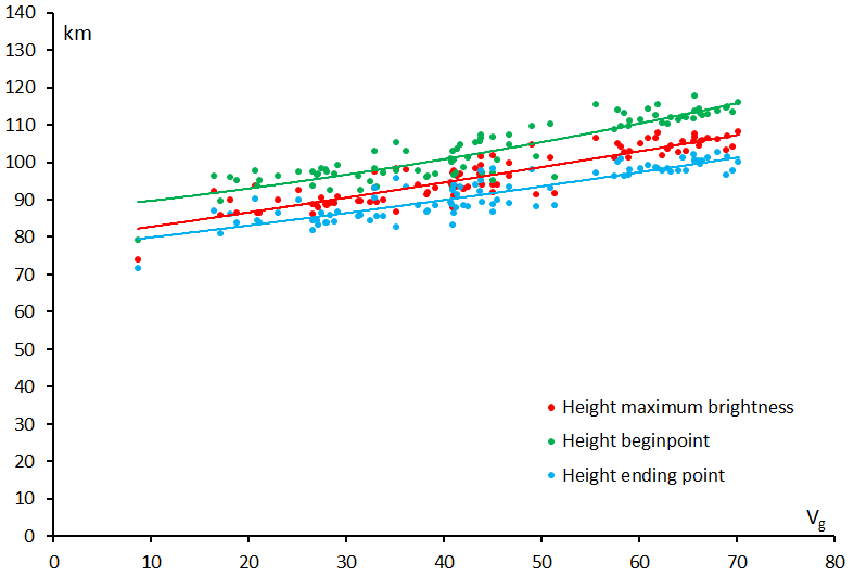
Figure 8 – The median values for shower meteors for the starting height (green), the height of maximum luminosity (red) and the ending height (blue) against the geocentric velocity.
A query selecting the orbits for all the established meteor showers that were present in the CAMS dataset allowed to compute the median values for the heights for the shower meteors. The shower identification in the dataset we use has been done by Dr. Peter Jenniskens and the method used has been described in a recently published paper (Jenniskens et al., 2016). The results are listed in Table 3 and in Figure 8. A number of meteor showers have a median value for the height of maximum brightness below 90 km, including one of the most active showers, the Geminids (GEM – 4). The terminal heights for meteor streams with low geocentric velocity is often closer to 80 km than to 90 km.
There is one extreme case for the Corvids (COR – 63) with their exceptional low geocentric velocity of 8.7 km/s for which the trajectories appear well below the 80 km level. So far this is the only meteor stream known with such extremely slow meteors. If we want to make sure that the network has no gaps where these Corvids can be missed, we should optimize at 70 km. This would require more cameras to cover the atmosphere above the BeNeLux than currently available. Considering the exceptional nature and the poor activity level of the Corvids, the tradeoff between costs for more cameras and the gain in number of orbits favors a compromise at a level of 80 km to optimize the overlap between the camera fields.
6 Conclusion
The statistics derived from the CAMS 2010–2013 dataset show a seasonal variation in the median value of the geocentric velocity and the related height of the ablation of sporadic meteors. A count of heights in 5 km thick layers indicate two levels with high numbers of events with in between a layer with remarkable less events. The median values for the sporadics and all shower meteors would favor the 90 km level to optimize the camera fields. When we look at the statistics for the individual meteor showers we have to use the 80 km level to avoid creating any bias that could have a negative effect on the number of orbits derived for meteor showers with a low geocentric velocity.
References
Jacchia L., Verniani F., Briggs R. E. (1967). “An Analysis of the Atmospheric Trajectories of 413 Precisely Reduced Photographic Meteors”. Smithsonian Contributions to Astrophysics, 10, 1–139
Jenniskens P., Gural P. S., Dynneson L., Grigsby B. J., Newman K. E., Borden M., Koop M. and Holman D. (2011). “CAMS: Cameras for Allsky Meteor Surveillance to establish minor meteor showers”. Icarus, 216, 40–61.
Jenniskens P., Nénon Q., Albers J., Gural P. S., Haberman B., Holman D., Morales R., Grigsby B. J., Samuels D. and Johannink C. (2016). “The established meteor showers as observed by CAMS”. Icarus, 266, 331–354.
Porubcan V., Bucek M., Cevolani G. and Zigo P. (2012). “Variation of Meteor Heights and Solar-Cycle Activity”. Publications of the Astronomical Society of Japan, 64, id.86, 5 pages.


